BRAINPORT
Simulation Transferability
1 Mathematical Definitions
o simulate demand responsive transit (DRT) vehicles in the macroscopic simulation suite Urban Strategy [1], three main models are used: a mode choice model for determining which people will use a DRT (as opposed to private car, public transport or cycling), a DRT model handling DRT trip requests by assigning passengers to vehicles using a vehicle dispatcher, and a traffic assignment model responsible for computing the routes taken by both private car and DRT vehicles, resulting in (congested) travel times used as input in the mode choice model.
1.1 Mode choice model
The mode choice model (New Mobility Modeller) is specifically developed to explore the mobility impacts of connected and automated driving and shared mobility, using a multinomial logit model for mode choice estimation [2]. The core mathematical formula is based on the concept of utility: a theoretical construct defined as what the individual seeks to maximize. For each alternative travel option (i.e., mode), for each alternative population group (e.g. representing characteristics such as car possession, income levels, etc.), the utility is computed using a generalized cost function.
The generalized cost function GC for each mode and population group used in the New Mobility Modeller is provided below:
Where,
- βtime = scalar weight of the attribute travel time.
- Time=TravelTime+WaitingTime+ ParkingTime
- TravelTime = the travel time of the mode for the specific trip (Origin-Destination-pair). For public transport, this also includes the time needed to walk or cycle to/from the public transport stop as well as waiting time between different public transport lines.
- WaitingTime = the time it takes (on average) before the vehicle arrives.
- ParkingTime = the time it takes (on average) to find a parking place and walk to the destination, for the specific destination zone.
- βcost = scalar weight of the attribute travel cost.
- Cost=CostStart+(TravelDistance * CostDistance)+ParkingCost
- CostStart = Cost associated for using the mode, independent of the actual kms travelled.
- TravelDistance = the travel distance of the mode for the specific trip (Origin-Destination-pair).
- CostDistance = Cost associated per km travelled by the travel mode, for example the fuel costs per km.
- ParkingCosts = the costs of parking at the destination zone
- ASCmode_popugroup is the Alternate Specific Constant per mode and per population group.
Using the Generalized Cost calculation, the utility per mode and population group alternative is obtained and used in computation of the mode probability per group, using the Multinomial logit equation provided below:

The probability is multiplied by the total number of trips for each Origin-Destination pair. Additionally, certain constraints are being set beforehand to specify which population groups may use which modes. For example, it is required to own a drivers license and a car to be able to use the private car as a mode on your trip.
1.2 Demand Responsive Transit model
The DRT model is responsible for assigning passengers to cars using a vehicle dispatcher. The model uses a relatively simple greedy algorithm [3]:
- Sort all trip requests on request time (earliest first) and travel distance (longest first)
- For each trip request:
- Find the closest (idle) DRT vehicle
- Assign DRT vehicle to trip request
- Update DRT vehicle location and availability according to the trip planned.
It is assumed that every DRT vehicle can only carry one passenger. Additionally, the fleet size is set as an input parameter, including the starting position of the vehicles. The resulting average waiting time for each Origin-Destination pair (i.e., time required to be picked up by a vehicle) is used as an input in the mode choice model.
Traffic assignment model
The traffic assignment model assigns private cars and DRT vehicles to the car network. This possibly results in congestion, and thereby updated travel times. These travel times are used in the mode choice model and influence the mode choices made by people.
The traffic assignment model uses a Volume Averaging Algorithm, also known as the Method of Successive Averages (MSA) [4]. This algorithm assigns traffic to the network using an iterative process. The volume on each road link is calculated as a linear combination of part of the volume computed in the previous iteration, and part of the volume by means of assigning traffic to the current best routes. By default, in each iteration of a volume-averaging assignment, the fraction 1/n is used to increase the link volume and the value (1-1/n) to reduce it, with n being the number of iterations.
The travel times on each road link are computed using the BPR function, as specified below:
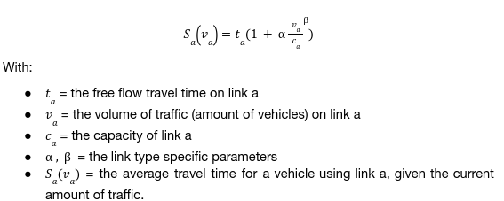
The Volume Averaging algorithm procedure then looks as follows:
- For each iteration n
- Find the shortest path for each Origin-Destination pair in the network
- “Shortest path” is hereby defined as the path where Traveltime*VoT+Traveldistance*VoD is minimized, with VoT and VoD being parameters set beforehand. This means that the best route is a combination of the fastest and shortest route. For example, one will not take a detour of 30km for a 1 minute shorter travel time.
- In the first iteration, this is based on free flow (uncongested) travel times. In the next iterations, this is based on the travel times computed using the BPR function.
- Reassign 1/n amount of traffic according the current fastest shortest path
- Recompute the link costs using the BPR function
This results in a traffic assignment that approaches an equilibrium situation, that is, a situation where no one can improve their travel time by switching to another route.
2 Parameterization
In the previous chapter, various formulas and accompanying parameters were introduced for the three main models: mode choice, demand responsive transit (vehicle dispatching) and traffic assignment. This chapter describes the values of the parameters used for each of these model, including adopted variations for several scenarios.
2.1 Mode choice model
The mode choice module (New Mobility Modeller) is specifically developed to explore the mobility impacts of connected and automated driving and shared mobility, using a multinomial logit model for mode choice estimation [2]. The core mathematical formula is based on the concept of utility: a theoretical construct defined as what the individual seeks to maximize. For each alternative travel option (i.e., mode), for each alternative population group (e.g. representing characteristics such as car possession, income levels, etc.), the utility is computed using a generalized cost function.
The generalized cost function GC consists of several components. For the default scenario, the values used are shown in Table 1.
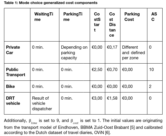
- Cost variations for DRT:
- Default: €3 + €1.58 per km
- Cheap: €1.50 + €0.50 per km
- Discouraging long trips: €1 + €3 per km
- Expensive: €4 + €3 per km
- ASC (attractiveness) variations for DRT:
- Default: 0 (based on private car)
- Less attractive: 1
- Least attractive: 2
2.2 Demand Responsive Transit model
The DRT model uses the fleet size and the location of the DRT vehicles as an input. Five starting locations of DRTs are selected and used in each of the scenarios (see Figure 1): Eindhoven Central train station, University, Strijp-S and two roads that are on the edge of the centre of Eindhoven.
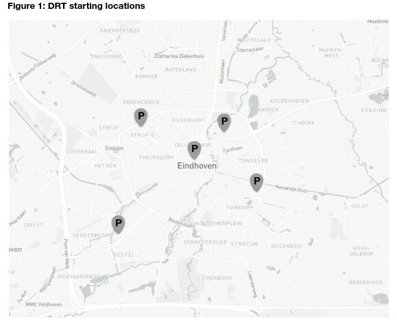
The different DRT scenarios vary by the number of DRT vehicles in the model:
- Base: 1000 vehicles (200 per location)
- “unlimited” (10 000 per location)
- 800 vehicles (160 per location)
- 600 vehicles (120 per location)
- 400 vehicles (80 per location)
- 200 vehicles (40 per location)
2.3 Traffic assignment model
In the traffic assignment model, the network including speeds and capacities are taken from the Eindhoven transport model [5]. It is assumed that DRT vehicles drive the same speed as private cars.
The BPR function is used to determine the link travel times. This function has specific and parameters that differ per link type. These are shown in Table 2 and taken from the Eindhoven transport model [5].
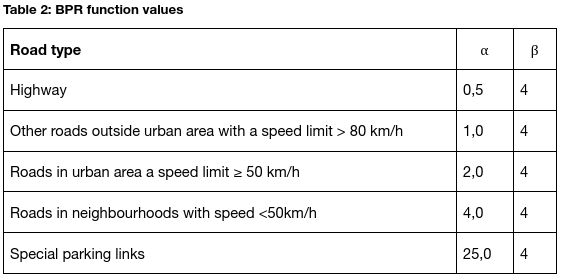
Additionally, a Value of Time (VoT) of €9,796 and a Value of Distance (VoD) of €0,078 is used to compute the best path. In total, 20 iterations are used for the Volume Averaging (MSA) algorithm.
The delays experienced at junctions by private cars are adopted from the Eindhoven transport model, which are computed using a sophisticated junction modelling algorithm with different delay functions for all junction types (signalized, unsignalized, roundabout, etc.) [7]. For the combination with DRT vehicles, several junctions were modelled in microscopic simulation environment VISSIM. The respective junction delays were adjusted. Additionally, also a scenario was run in VISSIM where DRT vehicles were prioritized and did not experience any delay. This results in the following three scenarios:
- Only junction delays as computed by the Eindhoven transport model.
- Original signalized junction delays adjusted to a situation where DRTs are driving around (using VISSIM results).
- Original signalized junction delays adjusted to a situation where DRTs are driving around and get priority (using VISSIM results).
3 Transferability
The Urban Strategy simulation tool applied at the Eindhoven region is a city level model. Urban Strategy and its models can also be applied in other cities, as long as there already exists a macroscopic transport model of the designated city which can be used as a starting point. Of course, the models themselves (especially the mode choice model) need to be calibrated to the newly modelled city.
The tooling provides the demand (e.g. amount of vehicles) for Demand Responsive Transit vehicles as one of the output values. This value can be used in microscopic simulation suites as an input: both for composing an Origin-Destination matrix at junction level, as well as the percentage of automated vehicles that can be expected on the road. This can help to design traffic infrastructure such that it is able to accommodate the (autonomous) vehicles in future. On the other hand, the microscopic simulations can be used as an input for macroscopic simulations in terms of junction delays or average speeds driven by the different vehicle types – as was also done in this Eindhoven study.
References
- Lohman, W., Cornelissen, H., Borst, J., Klerkx, R., Araghi, Y., & Walraven, E. (2023). Building digital twins of cities using the Inter Model Broker framework. Future Generation Computer Systems, 148, 501-513.
- Snelder, M., Wilmink, I., van der Gun, J., Bergveld, H. J., Hoseini, P., & van Arem, B. (2019). Mobility impacts of automated driving and shared mobility. European Journal of Transport and Infrastructure Research, 19(4).
- van der Tuin, M.S., Spruijtenburg, S.D., & Zhou, H. (2022). Vehicle dispatching in macroscopic transport models: modelling Demand Responsive Transit. Proceedings of Transport Research Arena 2022, Lisbon.
- de Dios Ortúzar, J., & Willumsen, L. G. (2011). Modelling transport. John wiley & sons.
- Provincie Noord-Brabant (2018). BrabantBrede ModelAanpak – model Zuid Oost Brabant.
- Centraal Bureau voor de Statistiek (2010-2017). Onderzoek Verplaatsingen in Nederland (OViN).
- DAT.Mobility (2016). Junction Modelling in OmniTRANS