SALZBURG
Simulation Transferability

1 Mathamatical Definitions
To integrate automated driving vehicles in the microscopic simulation environment of MATSim, several functions were adjusted and parameters of the MATSim model were changed. In general, automated vehicles do not behave differently to other vehicles in the MATSim model apart from different maximum speeds. This is due to the queuing models that are applied in MATSim for the traffic simulations. Detailed models for car following or lane changing are not part of MATSim. Overtaking of slower vehicles is possible in MATSim, but this is done in a simple fashion by changing the positions of vehicles in the queue on a link (see e.g. Horni et Al. 2016).
The main aspect of using MATSim for the simulation of automated vehicles is, that it allows the estimation of changes of demand in a transport system once automated vehicles are introduced. This is done by changing the scoring functions in MATSim (see e.g. Horni et Al. 2016). However, useres react differently to automated vehicles, using different values of travel time savings (VTTS). For this, the Charypar-Nagel Utility Function is used in the current model (see section 3.2 in Horni et Al. 2016).
Horni, A, Nagel, K and Axhausen, KW(eds.) (2016). The Multi-Agent Transport Simulation MATSim. London: UbiquityPress. DOI:http://dx.doi.org/10.5334/baw.
Mode Choice Model Parameters in the Charypar Nagel Utility function
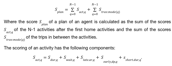
According to (Horni et Al. 2016) the basic scoring function of the MATSim simulation model is given as

The first term stands for the utility of performing a task, the second for waiting for an activity, e.g. when the shop is still closed, the third for a late arrival at an activity, the forth for a necessary early departure from the activity and the last for the disutility if the duration of the activity is too short.
For the current model in Salzburg, the activity scoring remains mostly unchanged compared to the default parametrization of the MATSim model. The only changes are done for the scoring of the waiting activity that MATSim introduces at the beginning of each public transport and DRT-leg. Here parameters for late Arrival, waiting and waitingPt are set manually. According to the meta-analysis by Wardman et al. [1], the disutility for arriving 10 minutes too late at an activity amounts on average to 1.9 times the disutility associated with a 10-minute increase in in-vehicle time, whereas waiting for a facility to open is penalized by 1.83 times pt-in-vehicle time, and waiting for public transport by 1.77 times pt-in-vehicle time. In accordance to the implementation in MATSim (Axhausenetal.[2] p.29), we therefore set

In the remainder of the description, we concentrate on the scoring of the trips between the activities. Here we concentrate on the scoring of the trips in between the activities.
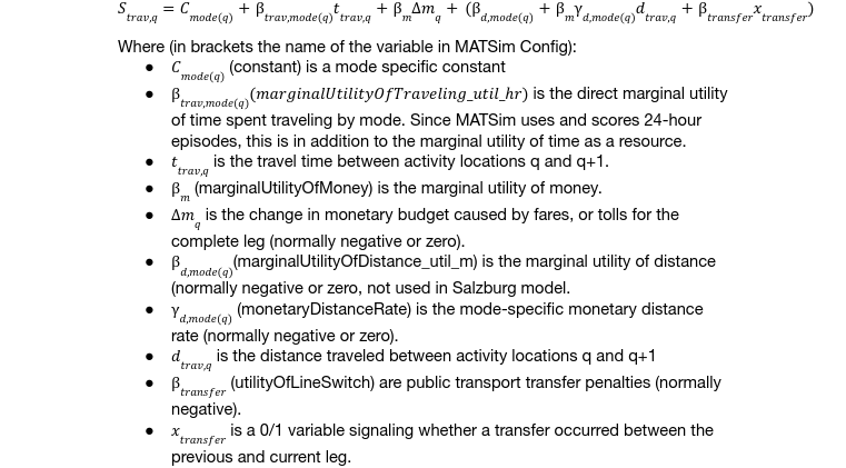
Travel disutility for a leg q is given in Horni et Al 2016 as

In the Salzburg model the disutility depending on the distance was not used.
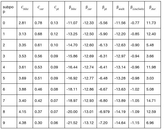
To allow for differences of behaviour in different groups of the population, 10 subpopulations were defined. For each subpopulation, we derive a distinct set of parameters that is used in the scoring function of the MATSim model [2] and the model calibration. More specifically, the mode-specific constants, the value of travel time savings (VTTS), the Value of Leisure (VoL), and the disutility associated with transfers vary across sub-populations. Note that the VTTS equals the VoL (i.e., opportunity costs of time) minus the direct utility (or disutility) derived from the time spent traveling (which typically depends on travel conditions such as crowding, comfort, and the possibility to use the travel time productively).
The parameters of the subpopulations are derived from the Mobility-Activity-Expenditure Diary data described in [3]. This data source contains a weekly mobility and activity diary as well as expenditures from a representative sample of Austrians. In addition, stated preference data on hypothetical mode choice situations from the same individuals have been collected. The detailed data do not only allow for the estimation of the VTTS and other mobility-related preference parameters, but also for the estimation of the VoL, which is the marginal utility associated with those activities to which more time than the necessary minimum is assigned (such as leisure activities). The empirical model follows the theoretical framework developed by [4]
Estimating of the VoL requires fitting the observed expenditures and time use patterns against the utility-maximization framework developed by Jara-Diaz and co-authors, using maximum likelihood estimation. The VTTS and other travel-related preference parameters, in contrast, can be derived from a (discrete) mode choice model applied to all trips contained in the sample. For the Austrian data set, these estimations have been performed separately (the VoL estimation can be found in [3] and the VTTS estimation in [7]), but also jointly in[5], which has the advantage that correlations between time use, expenditure and mode choice behaviour can be accounted for in a coherent way. The parameters used in this paper are also derived from a joint estimation, albeit somewhat different from [5] to simplify how socioeconomic characteristics can be combined into subpopulations. The parameters presented here are derived from a Latent Class Model – a classification model to assign observable discrete variables to latent classes (see for instance [6]), in which all model components are connected via a joint likelihood function and an overarching class membership equation.
The mode choice model that is part of the joint estimation is a more parsimonious version of the model presented in [7], and uses actual and hypothetical trip data. The time use and expenditure equations are estimated in a similar way as in [3] and [5]. We estimate two classes of coefficients for all parameters, since not much explanatory power is gained by introducing more classes. The class membership equation then determines for each individual the class membership probability, i.e. how much weight each class of coefficients has for a specific person. The class membership probability in turn is a linear function of several binary socioeconomic variables sex, age below 35, age above 55, income higher than median, education high-school or above, living in urban area, kids living in the household, single household, and full-time work with at least 38 hours a week. These socioeconomic variables were chosen since they were available both in the estimation data as well as in the synthesised population. An exception is the high-income variable for which the self-reported living standard was used as a proxy.
The demand-responsive transportation (DRT) Fleet was implemented in the simulation by using MATSim’s drt module. These vehicles are planned as automated, electric vehicles with a maximum capacity of 4 passengers. Ridesharing will be executed in case there are ride requests in the proximity of the vehicle and the the agents’ destinations do not differ too much.
For each of areas in the scenarios we assume that there is only one fleet operator with one price scheme operating as door2door service. The actual implementation of such a DRT fleet in real life is difficult to predict as fully-automated vehicles [9] will not be available for city traffic for another 10 years [10].
This is the reason why several parameters relevant for the operation of the fleet (e.g. base fare, minimum fare) could not be chosen based on a business model of an actual fleet operator but were disregarded instead. We assume that there will be a rebalancing of the DRT vehicles every 30~minutes based on the demand which is aggregated over cells with a size of 500~m. The SAEV vehicles are randomly distributed across the simulation area. Idle vehicles will return to one of these starting locations as they are regarded as depots. At the beginning of each simulation iteration, the SAEV vehicles will again start from these predefined, random locations.
The DRT rides are simulated on MATSim’s car network.
The maximum waiting time is set to 10 minutes. If this waiting time is exceeded, the request will be rejected. For boarding and disembarking the DRT vehicle one additional minute of travel time is added. The logic of the simulation is that an agent only requests a DRT vehicle as soon as the previous activity has finished. Then the scheduler of the drt module assigns a vehicle to the agent. This means that agents always have to wait for the DRT pickup.

2 Parameterization
In a mesoscopic model, that relies on queuing models, driving behaviour of automated vehicles does not differ significantly from that of other vehicles on the road, apart from slower maximal speeds. These are part of the MATSim
There are two ways to include automated public transport. The first is to add shuttles that run on schedule by adding them to the General Transit Feed Specification (GTFS) that is used to include public transport to the MATSim Model. The public transport vehicles can then either be included Hence, the main parametrization of the model happens in the DRT model, that enables MATSim to match agents with vehicles for parts of their trips. For the assignment of DRT vehicles to agents, the MATSim DRT Module was applied, which contains a matching algorithm described in Bischoff et Al. 2017 [8]

The costs for driving and owning a car follow estimations by [11] for average vehicles and are considered by setting dailyMonetaryConstant to $-13.521$ and monetaryDistanceRate to $0.00009$ ($0.09$ EUR/km). Costs for cycling were estimated as 1 EUR/day based on [12]. The travel costs for public transport were manually configured by averaging fares from station to station. This results in costs of $1.60$ EUR/day in Vienna ($0.67$ EUR/day for trains) and $1.38$ EUR/day (and additional $0.15$ EUR/km) outside of Vienna.
The costs associated with SAEVs consist of time costs as well as fares (the latter differ across scenarios and will be specified when introducing the scenario). In line with several studies, we assume that the VTTS associated with riding a SAEV is similar to the VTTS of car passenger: whereas [13] found no differences in the VTTS between drivers and passengers of a car [14], [15,16,17] come to the conclusion that the VTTS for a passenger decreases by 18%-30%. We follow in our model these latter findings and assume the VTTS for passengers in automated vehicles to be 75% of that of car users.
When applying the methodology to a new site, the model needs to be adjusted, using a new graph, a new population and by calibrating the constant parameters in the mode choice model. In the current setting this was done in the following way:
The model was calibrated by the modal split per trip that was taken from “Österreich Unterwegs 13/14” [19]. By adjusting the constants along all subpopulations we achieved a simulation equilibrium with a deviation of the modal split by trips of less than 1 % for each mode. The modal split per kilometer also deviates only by a few percentages. This rather good fit was the result of an a priori selection of activity locations that optimally fit the activity chains and the corresponding reported travel times and distances from “ÖU13/14”. Cadyts [18] was used simultaneously during the search for optimal constant parameters to align the simulated traffic volumes with the measured traffic counts.
3 Transferability
The Salzburg MATSim model is at city level. MATSim is designed to deliver in depth information on demand, both modal split but also the detailed assignment of vehicles and agents to routes. This gives a good opportunity to use MATSim output as an import source for microscopic simulations, where demand is usually an input variable.
One of the outputs of MATSim is a detailed Events file that includes the times when vehicles leave and enter edges in the transport graph. This can be applied to create OD-Matrices for input intomicroscopic traffic simulations (e.g. SUMO via the od2trips function). One has to adjust the OD-Matrix data for the percentage of the population simulated in MATSim. In the Salzburg Scenario, 25% of the population were simulated, so the OD-Matrices need to be upscaled to 100% for the input into the microscopic transport simulation. Together with OD-Matrices, it is possible to extract complete routes for each vehicle. This might be a different way to import the demand data into microscopic simulations avoiding time consuming traffic assignment routines. Functions exist for example in SUMO to input route information from VISUM. However an interface between the MATSim events output and SUMO does currently not exist to the best of our knowledge.
References
- Wardman, M., V.P.K. Chintakayala and G.de Jong, Values of trave time in Europe: 29 Review and meta-analysis. Transportation Research Part A: Policy and Practice, Vol.94, 30 2016, pp.93–111.
- Axhausen, K., A. Horni, and K. Nagel, The multi-agent transportsimulation MATSim. 11 Ubiquity Press, 2016.
- Hössinger, R., F. Aschauer, S. Jara-Díaz, S. Jokubauskaite, B. Schmid, S. Peer, K. Axhausen, and R. Gerike, A joint time-assignment and expenditure- allocation model: value of leisure and value of time assigned to travel for specific population segments.Transportation, Vol. 47, No. 3, 2020, pp.1439–1475.
- Jara-Díaz, S. R.,M. A. Munizaga, P. Greeven, R. Guerra,and K. Axhausen, Estimating the value of leisure from a time allocation model. Transportation Research Part B: Methodological, Vol. 42, No. 10, 2008, pp.946–957.
- Jokubauskaite, S., R. Hössinger, F. Aschauer, R. Gerike, S. Jara-Díaz, S. Peer, B. Schmid, K. Axhausen, and F. Leisch, Advanced continuous-discrete model for joint time-use expenditure and mode choice estimation. Transportation Research Part B: Methodological, 20 Vol. 129, 2019, pp. 397–421.
- Greene, W.H. and D.A. Hensher, A latent class model for discrete choice analysis: contrasts with mixed logit. Transportation Research Part B:Methodological, Vol. 37, No. 8, 23 2003, pp.681–698.
- Schmid,B.,S. Jokubauskaite, F. Aschauer, S. Peer, R. Hössinger, R. Gerike, S.R. Jara- Diaz, and K. Axhausen, A pooled RP/SP mode,route and destination choice model to investigate mode and user-type effects in the value of trave lime savings. Transportation Research Part A: Policy and Practice, Vol. 124, 2019, pp.262–294.
- Bischoff, Joschka, Michal Maciejewski, and Kai Nagel. “City-wide shared taxis: A simulation study in Berlin.” 2017 IEEE 20th international conference on intelligent transportation systems (ITSC). IEEE, 2017..
- Maurer, M., J. Christian Gerdes, B. Lenz, and H. Winner, Autonomes Fahren: technische, rechtliche und gesellschaftliche Aspekte. Springer Nature, 2015
- Wintersberger, S., M. Azmat, and S. Kummer, Are we ready to ride autonomous vehicles? A Pilot Study on Austrian Consumers’ Perspective. Logistics, Vol. 3, No. 4, 2019, p. 20.
- ADAC, ADAC Autokosten. https://www.adac.de/infotestrat/autodatenbank/
autokosten, 2020, online; retrieved on 24. July 2020. - DieEinsparBerater, Kosten-, Zeit- und Verbrauchsvergleich verschiedener Fahrradtypen. http://www.dieeinsparinfos.de/guenstige-mobilitaet/fahrrad/kosten/
uebersicht-energieverbrauch-und-kosten-beim-radfahren, 2020, online;
retrieved on 24. July 2020. - Lu, H., C. Rohr, B. Patruni, S. Hess, and H. Paag, Quantifying travellers’ willingness to pay for the Harbour Tunnel in Copenhagen: A stated choice study. MOE | Tetraplan, 2018
- Fosgerau, M., Automation and the value of time in passenger transport. International Transport Forum – ITF Discussion papers, 2019.