Graz

Simulation Transferability

1 Mathematical Definitions

For the integration of automated driving vehicles in the microscopic simulation environment a model is needed which approximates the real-world behaviour of the automated driving software in the simulation environment. Since two different simulators have been used for the Graz pilot site (SUMO, Autoware simulator), both are described in the following.

Car-Following Model

When simulating queued vehicles, car-following models are needed to emulate the acceleration behaviour of real vehicles. Depending on the model and the parameters, different vehicle gaps are the result. 

SUMO contains many car-following models which can be used to replicate automated driving in a simulated environment. For the SHOW project, the Intelligent Driver Model has been chosen for the shuttle operating at the Graz pilot site. Based on data recorded during the pre-pilot phase, this model approximates the speed profile best, both qualitative and quantitative.

The Intelligent Driver Model (IDM), first introduced as time-continuous model [Treiber2000], consists of two main equations and five parameters: the desired time headway T, the maximum acceleration amax, the desired deceleration bstandard, the minimum gap s0 and the acceleration exponent δ. The desired gap depends on the parameter amax, bstandard and T:

The latter ratio represents the intelligent braking strategy and assures a collision-free execution of this model. However, this term does not allow the following vehicles to reach the desired velocity in homogenous traffic condition and induces ever larger gaps. Because there is only one automated shuttle in the simulation, this drawback of this car follow model does not pose any problem. 

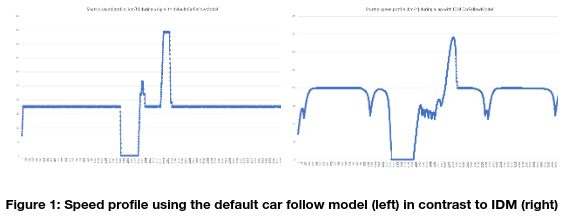
All other vehicles, like the individual traffic in the shopping center as well as the manual driven public busses, are using the default SUMO car-follow model. This model is extremely simple and can be calculated quickly for a large fleet of vehicles. Figure 1 compares the two models on one simulation run at the SHOW track in Graz. Obviously, the speed profile recorded using the default model (left) looks highly artificial while the IDM model (right) produces far more realistic speed profiles and smoother gradients.

Autoware uses an adaptive cruise controller module which embeds maximum velocity into the trajectory when there is a dynamic point cloud on the trajectory. The value of maximum velocity depends on the own velocity, the velocity of the point cloud (velocity of the vehicle ahead), and the distance to the point cloud which correspondences with the distance to the front car (see Figure 2).

The first process of this module is to estimate the velocity of the target vehicle point. The velocity estimation uses the velocity information of dynamic objects or the travel distance of the target vehicle point from the previous step. The dynamic object information is primal, and the travel distance estimation is used as a backup in case of the perception failure. If the target vehicle point is contained in the bounding box of a dynamic object geometrically, the velocity of the dynamic object is used as the target point velocity instead. Otherwise, the target point velocity is calculated by the travel distance of the target point from the previous step. Note that this travel distance based estimation fails when the target point is detected in the first time which may happen during a cut-in situation. To improve the stability of the estimation, the median of the calculation result for several steps is used.

If the calculated velocity is within the threshold range, it is used as the target point velocity. Only when the estimation succeeds and the estimated velocity exceeds the value of obstacle_stop_velocity_thresh, the distance to the pointcloud from self-position is calculated. For prevent chattering in the mode transition, obstacle_velocity_thresh_to_start_acc is used for the threshold to start adaptive cruise, and obstacle_velocity_thresh_to_stop_acc is used for the threshold to stop adaptive cruise. When the calculated distance value exceeds the emergency distance demergency calculated by emergency_stop parameters, target velocity to insert is calculated:

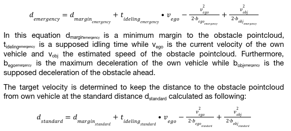
Therefore, if the distance to the obstacle pointcloud is longer than standard distance, the target velocity becomes higher than the current velocity, and vice versa. For keeping the distance, a PID controller is used.

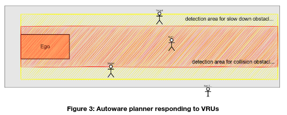
If there is a VRU detected in or near the planned trajectory, the so-called Slow Down Planner is activated. It inserts the slow down section before the obstacle with forward margin and backward margin. The ego vehicle keeps decelerating in the slow down section using the following equation:

As already mentioned in the Graz pilot site description, this Autoware simulation is primarily used for the traversal of the bus terminal where many VRUs are present. The majority of the track is covered by SUMO, as it is much better suited to simulate manual driven traffic in the shopping center.

Lane-Changing Model

At the Graz pilot-site no lane-changes in the usual manner are needed, because there are only single-lane roads. However, a decision is needed at the bus terminal, which lane through the terminal is currently available and must be chosen consequently. For this highly specific problem, a separate algorithm had to be developed, which is described briefly in the following section. It operates in the Autoware simulation domain only, since it needs a Lidar point-cloud as input – either from the simulator or from the real sensor. Based on the point cloud and the map of the bus terminal, an occupancy grid like structure is filled with data. 

In a first step the input data filtered depending on the height of the LiDAR points. In this case, only LiDAR points are considered, which are between 0.5 and 1.5 m, thus eliminating flickering of the ground and ignoring the structures of the building above. Furthermore, the raw data are filtered in 2D domain, and only points near the bus bays are considered.   

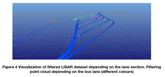
Figure 4 shows a sample view of LIDAR point clouds over a time sequence. Depending on the lane, LiDAR points are visualized with a specific color (the first bus lane in red, the second in green, and the third in blue). LIDAR points’ change over time (flow) has valuable information for deciding which lane to choose. The idea is to define the probability and uncertainty of a static and dynamic object by reading the LIDAR data. Therefore, we compute the probabilities as shown in in Figure 2.

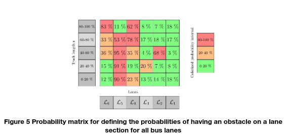
Figure 5 is only valid for a timestep. It is necessary to analyze the change in probability matrices over time. Especially for intelligent motion planning, the prediction over time is relevant.

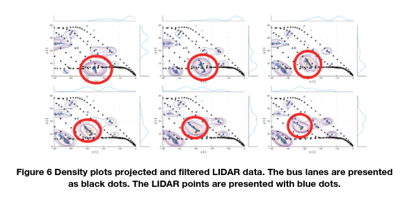
Figure 6 shows the filtered and projected dataset for a specific time sequence, where a bus is driving in bus lane 3. The visual shape of a bus (surfaces and edges) leads to typical patterns in LIDAR data. Occlusions by other road users or static objects might hide valuable information about the movements of all road users. This effect can be largely mitigated by including temporal evolution. Further details of this algorithm can be found in [1]. 

The intended usage of the presented algorithm is like the following: After picking up new passengers at the bus terminal, the test driver has to confirm that the shuttle is ready to start driving. During this human interaction the desired bus bay must also be specified. The algorithm shown above simplifies and accelerates this step by pre-selecting a reasonable bus bay. 

Sidenote: In the real world driving, an additional smart camera is used to aid this decision process and which triggers a TOR (Take Over Request) if no bus lane is available at all. 

Gap-Acceptance Model: Yield Behaviour

Besides basic models for longitudinal and lateral movement, a traffic simulation needs also models and algorithms to determine speed of a vehicle at intersections and for right-of-way rules. 

SUMO At most intersections, vehicles wait at the stop line at the border of the intersection until they may cross conflicting streams of traffic. The right-of-way model implemented in SUMO is a simplification of real world behavior: When approaching an intersection, a vehicle at first set the information about its approach to the intersection. After this has been done for all vehicles, the intersection decides which vehicles are allowed to pass without braking and which vehicles have to yield. This is done using a right-of-way matrix. This matrix describes which connections cross each other and which one has the right of way in case of crossing connections. This concept is illustrated in Figure 7 using an example.

Figure 7a shows an intersection which is approached by a red car on lane 2 and a green car on lane 7. Since the paths of both vehicles intersect and both wish to cross the intersection, a right of way computation is performed. In Figure 7b the right-of-way matrix for this intersection is shown, emphasizing the discussed links. The matrix cell with row i and column j defines the right of way for a vehicle on lane i in regard to a vehicle from lane j. According to the colors (white/yellow/red) a vehicle on lane i (ignores/has priority over/yields to) a vehicle on lane j. In the example, the red car yields to the green car because of the red box in cell (2,7) which agrees with the common rules of traffic for left-turning vehicles. So, we see that the vehicle at lane 2 has to wait for the vehicle at lane 7.

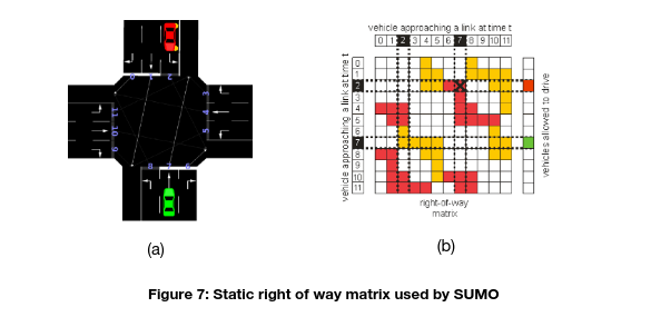
The matrix itself is static and computed during the network import/generation. Traffic lights are modelled by removing the information about approaching the intersection for all vehicles that run at links that have a red light.

Autoware. Unlike SUMO, where every vehicle is basically treated equally, Autoware always views the situation from an ego perspective. When approaching an intersection, only the ego lane is actually known; the behavior of other road users can only be extrapolated based on a HD map and/or guessed. 

Figure 8 depicts the situation when turning left at a T-crossing. The attention area in the intersection is defined as the set of lanes that are conflicting with ego vehicle’s path and their preceding lanes. Objects that satisfy the following conditions are considered as possible collision objects:

• center of gravity of the object is within a certain distance from the attention lane
• posture of object is the same direction as the attention lane 
• not being in the adjacent lanes of the ego vehicle
• not forced to stop by traffic light (if present)

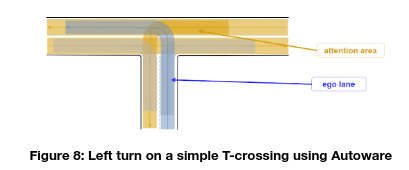
Figure 8: Left turn on a simple T-crossing using Autoware

The following process is performed for all target objects, to determine whether the ego vehicle can pass the intersection safely. If it is judged that the ego vehicle cannot pass through the intersection with enough margin, a stop-line is inserted in the path.

1. calculate the time interval that the ego vehicle is in the intersection. This time is set as ts ~ te
2. extract the predicted path of the target object
3. detect collision between the target extracted predicted path and ego’s predicted path in the following process.
1. obtain the passing area of the ego vehicle Aego in ts ~ te
2. calculate the passing area of the target object Atarget at ts-tmargin ~ te+tmargin for all predicted, possible paths
3. check if Aego and Atarget polygons are overlapped → collision
4. when a collision is detected, a stop-line is inserted

In a sense, it can be concluded that Autoware is much closer to human behavior than SUMO, because the uncertainties regarding other road users are also taken realistically into account. On the other hand, Autoware only has to work for a single ego vehicle, while SUMO has to make decisions for an entire fleet of vehicles in parallel.

2 Parameterization

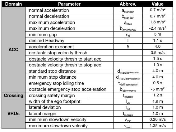
The parameters along with their definition that were adjusted for modelling automated vehicles for the present use case are listed in this chapter with their specific value specified in Table 1. Manually driven vehicles use default parameters for the individual vehicle class predefined in the simulation environment. 

• Normal acceleration (astandart): is the normal acceleration, in m/s2, that is used for normal, convenient driving.
• Normal deceleration (bstandart): is the normal deceleration, in m/s2, that the vehicle uses under normal conditions for convenient stopping.
• Maximum acceleration (amax): is the maximum acceleration, in m/s2, that the vehicle can achieve under any circumstances
• Maximum deceleration (bemergency): is the most abrupt braking, in m/s2 that the vehicle can apply in emergency situations.
• Minimum gap (s0): is the space, in m, between the rear bumper of a vehicle and the front bumper of the following vehicle.
• Desired Headway (T): the minimum allowed time, in s, to the vehicle driving in front 
• Acceleration exponent (δ): specifies how the acceleration decreases when approaching the desired velocity
• Obstacle stop velocity thresh: threshold, in m/s, for velocity of obstacle ahead to insert a stop line
• Obstacle velocity thresh to start acc: start adaptive cruise control when the velocity, in m/s, of the forward obstacle exceeds this value
• Obstacle velocity thresh to stop acc: stop adaptive cruise control when the velocity, in m/s, of the forward obstacle falls below this value 
• Standard stop distance (dmarginstandard):  is the normal margin, in m, to the obstacle pointcloud. Below this threshold convenient deceleration begins
• Minimum stop distance (dmarginemergency):  is the absolute minimum margin, in m, to the obstacle pointcloud. Below this threshold an emergency stop is initiated.
• Emergency stop idling time (tidelingemergency): is the supposed idling time, in s, to start an emergency stop
• Obstacle emergency stop acceleration (bobjemergency): assumed maximum deceleration, in m/s², of vehicle ahead during emergency stop 
• Crossing safety margin (tmargin): time safety reserve, in s, when driving through an intersection
• Width of the ego footprint (lvw): ego vehicle width, in m
• Lateral deviation (lld) between the obstacle and the ego footprint, in m
• Lateral margin (lmargin) for passing a VRU, in m 
• Minimum slowdown velocity (vmin): the minimum velocity, in m/s, within a slowdown section because of a VRU
• Maximum slowdown velocity (vmax): the maximim velocity, in m/s, within a slowdown section because of a VRU

2 Transferability

Since the Graz Pilot Site is very special in its configuration (passage of bus terminal, usage of restricted bus lanes, interaction with tramway), we cannot see the point of scaling up the simulations made there to the entire city of Graz or replicating them in this exact same way at another location.

For the present use case only microscopic simulations were conducted. Therefore, the application of an up-scaling methodology is necessary in order to conduct any transferability analysis of the results or any generalization with some degree of success. These types of methodologies are described in the following.

Up-scaling from micro to macro simulation using PCUs

A methodology of up-scaling automated driving simulation outputs, was conducted by Tympakianaki et al. (2022) [6] and used in the LEVITATE project (LEVITATE EU, 2022 [7]). In this methodology, the impacts of CAVs were assessed with respect to network performance. In [2] the considered steps of the up-scaling method are illustrated.

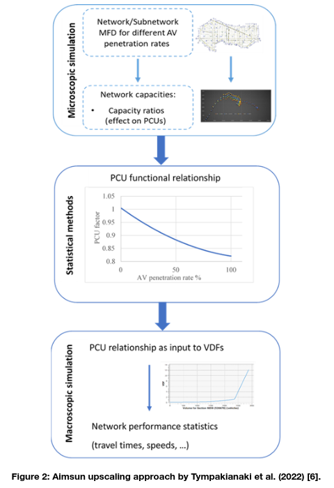
• The considered steps of the up-scaling method are explained: 

1. 1. Firstly, the network capacity should be derived through the microscopic simulation. By network capacity we define the maximum number of vehicles exiting the simulation network between simulation time intervals (e.g. 2 minutes). A suitable and easily transferable approach for observing the network capacities is through the Macroscopic Fundamental Diagram (MFD). The MFD is the basis of traffic flow theory and demonstrates a functional relationship between the network characteristics, i.e., traffic flow (throughput), vehicle density and speed.
   2. The second step includes a statistical analysis that identifies the effects on the Passenger Car Units (PCUs) as a relative change of capacities. Based on the microscopic simulation results, a fitted function (i.e. linear, polynomial, etc.) can be used to derive the PCUs given the capacities obtained from the network MFD. The PCUs are derived by the capacity ratio of conventional vehicles (CV) and AVs using the following formula: 

3. The last step is to provide the PCU relationship as an input to the Volume Delay Functions (VDFs) of macroscopic models to forecast the potential macroscopic implications on the network performance. The VDFs are functions that model travel time among different parameters such as volume and capacity. For this reason, the macroscopic models apply VDFs in order for travel time values to be calculated. VDFs represent the relationship between flows and delays of each road segment. A function defining travel time was developed by US Bureau Public Roads (1964) [8] and is the following:

where tff is the free-flow travel time, v/c is the volume-to-capacity ratio, and a, b two adjustable parameters.

This methodological approach is essential as the small-scale simulated networks would be up-scaled to city-level networks. In addition, the transferability of the simulation outputs to other networks or/and regions would be applicable. If a microscopic simulation model of a city is not available, the generalized PCU functional relationship estimated from a different network could be used as input into a travel demand model to forecast the macroscopic impacts. Furthermore, more robust simulations with validated automated driving parameters (limiting the assumptions related to the used parameters) could be executed and consequently, more concrete results could be extracted. 

This methodology requires the combination of micro with macro simulations. The main benefit of this methodology is that the results of microscopic simulation can be evaluated if are significantly similar to those derived from macroscopic simulation (essentially to be up-scaled) in order to see if they can be generalized as well as are transferable to different regions or cities. Therefore, the fundamental expected outcomes by applying this methodology are that up-scaled to city-level network results can be derived and this does not restrain the results only to micro and macro as well as this method gives the ability to the simulation outputs to be transferable to other networks/regions.

Up-scaling from micro to macro simulation using extensions of driver models and additional MFD specifications

Building upon the PCU method and recent advances in the literature with regards to traffic flow theory and AVs, the MFD could be further exploited for upscaling processes. One alternative is proposed by Shi and Li (2021) [9], where an MFD for AV traffic flows is proposed along with macroscopic and microscopic measurement proposals. For example, using vehicle travel time and distance travelled inside a simulation area, an MFD can be created and up-scaled in the macro scale, in order to be fitted into a macroscopic simulation. Furthermore, recently developed models such as the cell transmission model (CTM) by Adacher and Tiriolo, (2018) [10], headway modelling as described in Li and Chen, (2017) [11] and the Flexible Traffic Stream Model (FTSM) by Zheng et al. (2017) [12], that have been shown to be easily transferrable from the micro to the macro scale could be used to obtain MFDs using the methodology described in Lu et al., (2020) [13]. In Lu et al., (2020) [13], an MFD is drawn based on measurements from SUMO inputs and a macroscopic speed-density function is obtained through a Generalised Additive Model (GAM) regression for specific AV penetration rates.

As it can be understood, apart from network capacity and the PCU method, even with limited AV trajectories (as in Shi and Li, 2021 [9]) or with the exploitation of headways (Zheng et al., 2017 [12]) and speeds of vehicles (Lu et al. 2020 [13]) the transferability of microscopic simulation outputs can be achieved through the construction of MFDs to the macroscopic level and further impact assessment results can be obtained.

References

[1] M. Hartmann, J. Hillebrand, D. Watzenig and S. Fernandes. 2023. LiDAR perception for automated vehicles in frequented public areas with buses and VRUs. In Proceedings of the 15th Intelligent Transport Systems European Congress (ITS) 2023, May 22-24, Lisbon, Portugal.