MADRID
Simulation Transferability

1 Mathematical Definitions
To integrate automated driving vehicles in the microscopic simulation environment of Aimsun software, several parameters of the implemented in the software driving models were adjusted. Information regarding the driving models are follow based on the Aimsun Next User’s Manual (22.0.1) [1] focusing mainly on the parameters that were adjusted for modelling automated driving vehicles.
Car-Following Model
The Aimsun software incorporates the Gipps car-following model, originally formulated by Gipps (1981) [2], which analyzes the behavior and reaction of the following vehicle in relation to the actions of the preceding vehicle. This model considers specific parameters that are not universally applicable but rather depend on local factors such as the driver’s characteristics (e.g. acceptance of speed limits), section geometry (e.g. speed limits on the section and turns), and the influence of vehicles in neighboring lanes, among others.
According to this model, the desired speed (V*) of vehicle (n) in section (s) is determined as follows:

In addition, this model comprises two elements: acceleration and deceleration. The acceleration component reflects a vehicle’s intent to reach a specific desired speed, whereas the deceleration component replicates the constraints imposed by the preceding vehicle when attempting to travel at the desired speed. The maximum acceleration speed (Va) that a vehicle (n) can attain within a given time period denoted as (t, t+T) is expressed as follows:

Simultaneously, the maximum speed (Vd) that the vehicle (n) can achieve within the same time interval (t, t+T), taking into account its individual characteristics and the constraints imposed by the presence of the preceding vehicle (vehicle n-1), can be defined as follows:


The speed (V) for vehicle n within the time interval (t, t+dt) is determined as the minimum value between these two speeds:
The position of the vehicle n within the current lane is recalculated by integrating the speed. The integration process for the acceleration and deceleration phases employs distinct methods. Specifically, the acceleration phase is integrated using the rectangle method, which can be expressed by the following equation:
while the integration of the deceleration phase employs the trapezoid method, which is characterized by the following equation:
Lane-Changing Model
The lane-changing model integrated into the Aimsun software builds upon the Gipps lane-changing model [3], encompassing additional features and functionalities. Lane changes are represented as a decision-making process, considering factors such as the necessity of changing lanes (e.g. for turn maneuvers as determined by the route), the desirability of the lane change (e.g. to attain the desired speed when the leading vehicle is slower), and the feasibility of the lane change based on the vehicle’s position in the road network, lane geometry, and surrounding vehicles.
Lane-Changing zone distance calculation
Lane-changing zones are defined by two parameters: look-ahead and critical look-ahead. The look-ahead represents the distance upstream from the vehicle’s current position to the point where it becomes aware of its target lanes. On the other hand, the critical look-ahead corresponds to the distance upstream to the starting point of the lane change. When these parameters are specified in terms of time, the conversion to physical distance is computed as follows:

Overtaking Manoeuvre
In the Aimsun software, an overtaking maneuver occurs when a vehicle, positioned within its set of permissible lanes, changes lanes to surpass another vehicle. To regulate and influence the frequency of overtaking, two parameters are employed:
- Overtake Speed Threshold is the percentage of the desired speed of a vehicle below which the vehicle might decide to overtake. This means that whenever a vehicle is constrained to drive slower than Overtake Speed Threshold % of its desired speed, it will try to overtake. The default value is 90%.
- Lane Recovery Speed Threshold is the percentage of the desired speed of a vehicle above which a vehicle will decide to get back into the adjacent slower lane. The default value is 95%.
Gap-Acceptance Model: Yield Behaviour
The Aimsun simulation software also incorporates a Gap-Acceptance model to simulate yielding behavior. This model determines whether a vehicle approaching an intersection can proceed or must wait based on the presence of other vehicles with higher priority at the junction. It considers factors such as the distances between vehicles and a hypothetical collision point, their speeds, and acceleration rates. Using this information, the model calculates the time required for vehicles to clear the intersection and produces a decision that also incorporates the level of risk for each driver.
When determining when a vehicle can move at a priority junction in the context of gap acceptance calculations, the “safety margin” is established in the road type turn related parameters. This safety margin can be adjusted to account for specific road geometry and can be further adjusted based on the vehicle type. This vehicle type parameter serves as a multiplier, within a truncated normal range, to modify the turn safety margin values. In addition, the behavior of the gap-acceptance model is influenced by several other vehicle parameters, including turn speed, acceleration rate, desired speed, and speed limit acceptance.
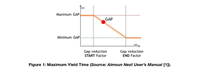
The gap required for executing a maneuver is determined by the duration of waiting for a suitable gap to appear in the opposing flows. The initial value is MaximumGap; the final value is MinimumGap. After waiting for GapReductionStartTime
* MaximumGap seconds, the gap is progressively reduced, reaching the minimum gap value after GapReductionEndTime * MaximumGap seconds as shown in following figure (Figure 1).

2 Parameterization
The parameters along with their definition that were adjusted for modelling automated driving vehicles for the present use case are the following:
- Maximum acceleration: is the maximum acceleration, in m/s2, that the vehicle can achieve under any circumstances.
- Normal deceleration: is the maximum deceleration, in m/s2, that the vehicle can use under normal conditions.
- Maximum deceleration: is the most abrupt braking, in m/s2 that a vehicle can apply under special circumstances, such as emergency braking for e.g. in front of a traffic light.
- Clearance: is the space, in m, between the rear bumper of a vehicle and the front bumper of the following vehicle.
- Overtake speed threshold: is the percentage of the desired speed of a vehicle below which the vehicle might decide to overtake. This means that whenever a vehicle is constrained to drive slower than Overtake Speed Threshold % of its desired speed, it will try to overtake.
- Look ahead distance factor: is the upstream distance, to the point where the vehicle is aware of its target lanes, expressed as a factor.
- Safety margin: is a factor which determines when a vehicle can move at a priority junction.
- Reaction time: is the time, in seconds, it takes a driver to react to speed changes in the preceding vehicle.
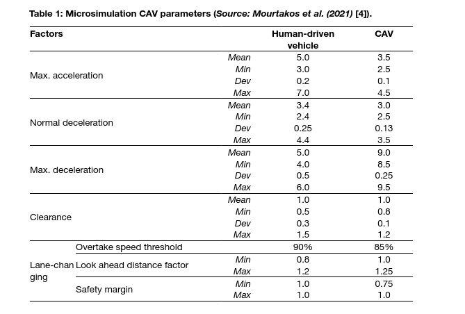
The parameter values for human-driven vehicles as well as automated driving vehicles are presented in the following table (Table 1).

As shown in the above Table, acceleration and deceleration of CAVs were selected to be slower than human-driven vehicles based on a study conducted by Karjanto et al. (2016), in order for in-vehicle activities (apart from driving) to be enabled for the users. Moreover, the “Look ahead distance” parameter, also known as “Distance zone factor” was also considered to be different between conventional vehicles and CAVs, because this parameter emulates connectivity in the sense that CAVs will have better knowledge of junctions and turnings. Therefore, it was considered that the modelled CAVs change lanes earlier than human-driven vehicles.
The “Reaction time” parameter is the parameter that concerns the reaction time in car-following and, along with sensitivity factor, affects time headway. According to Eilbert et al. (2019), Adaptive Cruise Control (ACC) applications seem to be bimodal, featuring either a gap setting of 1.1 seconds to eliminate cut-in vehicles or a 1.5 seconds gap likely due to not trusting the ACC system to be able to stop timely. For these reasons, ACC driving appears to have a higher average time gap than manual driving. Therefore, CAVs presented higher reaction time values compared to conventional vehicles. All the above vehicle parameters of Table 1 were presented in a recent study by Chaudhry et al. (2022) [5] and were based on a comprehensive literature review conducted within the LEVITATE project.
3 Transferability
For the present use case only microscopic simulations were conducted. Therefore, the application of an up-scaling methodology is necessary in order to conduct any transferability analysis of the results or any generalization with some degree of success. These types of methodologies are described in the following.
Up-scaling from micro to macro simulation using PCUs
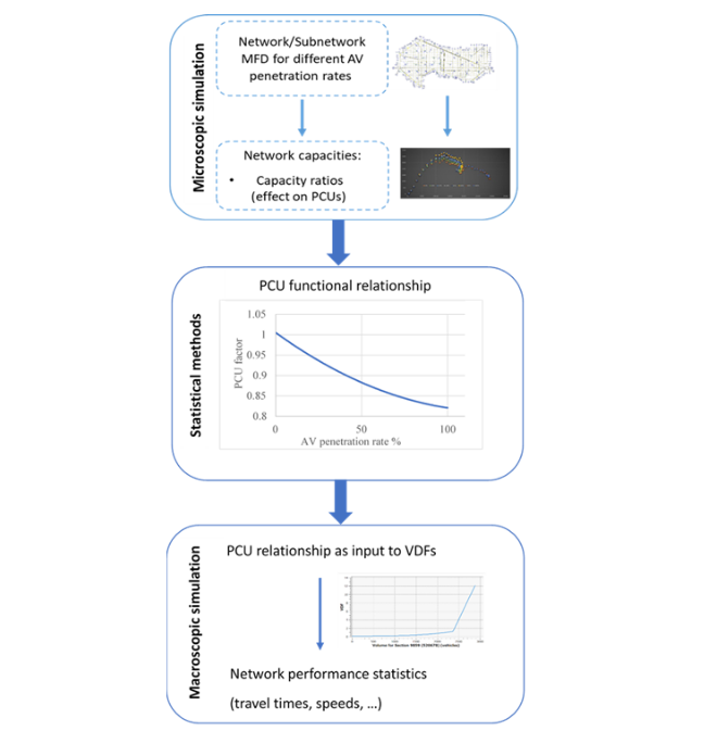
A methodology of up-scaling automated driving simulation outputs, was conducted by Tympakianaki et al. (2022) [6] and used in the LEVITATE project (LEVITATE EU, 2022 [7]). In this methodology, the impacts of CAVs were assessed with respect to network performance. In Figure 2, the considered steps of the up-scaling method are illustrated.

Figure 2: Aimsun upscaling approach by Tympakianaki et al. (2022) [6].
The considered steps of the up-scaling method are explained:
- Firstly, the network capacity should be derived through the microscopic simulation. By network capacity we define the maximum number of vehicles exiting the simulation network between simulation time intervals (e.g. 2 minutes). A suitable and easily transferable approach for observing the network capacities is through the Macroscopic Fundamental Diagram (MFD). The MFD is the basis of traffic flow theory and demonstrates a functional relationship between the network characteristics, i.e., traffic flow (throughput), vehicle density and speed.
- The second step includes a statistical analysis that identifies the effects on the Passenger Car Units (PCUs) as a relative change of capacities. Based on the microscopic simulation results, a fitted function (i.e. linear, polynomial, etc.) can be used to derive the PCUs given the capacities obtained from the network MFD. The PCUs are derived by the capacity ratio of conventional vehicles (CV) and AVs using the following formula:

3. The last step is to provide the PCU relationship as an input to the Volume Delay Functions (VDFs) of macroscopic models to forecast the potential macroscopic implications on the network performance. The VDFs are functions that model travel time among different parameters such as volume and capacity. For this reason, the macroscopic models apply VDFs in order for travel time values to be calculated. VDFs represent the relationship between flows and delays of each road segment. A function defining travel time was developed by US Bureau Public Roads (1964) [8] and is the following:

This methodological approach is essential as the small-scale simulated networks would be up-scaled to city-level networks. In addition, the transferability of the simulation outputs to other networks or/and regions would be applicable. If a microscopic simulation model of a city is not available, the generalized PCU functional relationship estimated from a different network could be used as input into a travel demand model to forecast the macroscopic impacts. Furthermore, more robust simulations with validated automated driving parameters (limiting the assumptions related to the used parameters) could be executed and consequently, more concrete results could be extracted.
This methodology requires the combination of micro with macro simulations. The main benefit of this methodology is that the results of microscopic simulation can be evaluated if are significantly similar to those derived from macroscopic simulation (essentially to be up-scaled) in order to see if they can be generalized as well as are transferable to different regions or cities. Therefore, the fundamental expected outcomes by applying this methodology are that up-scaled to city-level network results can be derived and this does not restrain the results only to micro and macro as well as this method gives the ability to the simulation outputs to be transferable to other networks/regions.
Up-scaling from micro to macro simulation using extensions of driver models and additional MFD specifications
Building upon the PCU method and recent advances in the literature with regards to traffic flow theory and AVs, the MFD could be further exploited for upscaling processes. One alternative is proposed by Shi and Li (2021) [9], where an MFD for AV traffic flows is proposed along with macroscopic and microscopic measurement proposals. For example, using vehicle travel time and distance travelled inside a simulation area, an MFD can be created and up-scaled in the macro scale, in order to be fitted into a macroscopic simulation. Furthermore, recently developed models such as the cell transmission model (CTM) by Adacher and Tiriolo, (2018) [10], headway modelling as described in Li and Chen, (2017) [11] and the Flexible Traffic Stream Model (FTSM) by Zheng et al. (2017) [12], that have been shown to be easily transferrable from the micro to the macro scale could be used to obtain MFDs using the methodology described in Lu et al., (2020) [13]. In Lu et al., (2020) [13], an MFD is drawn based on measurements from SUMO inputs and a macroscopic speed-density function is obtained through a Generalised Additive Model (GAM) regression for specific AV penetration rates.
As it can be understood, apart from network capacity and the PCU method, even with limited AV trajectories (as in Shi and Li, 2021 [9]) or with the exploitation of headways (Zheng et al., 2017 [12]) and speeds of vehicles (Lu et al. 2020 [13]) the transferability of microscopic simulation outputs can be achieved through the construction of MFDs to the macroscopic level and further impact assessment results can be obtained.
References
- Aimsun Next Users Manual (22.0.1). (2023). Modeling Vehicle Movement. https://docs.aimsun.com/next/22.0.1/UsersManual/MicrosimulationModellingVehicleMovement.html
- Gipps, P.G., 1981. A behavioural car-following model for computer simulation. Transport. Res. Part B 15 (2), 105–111. https://doi.org/10.1016/0191-2615(81)90037-0
- Gipps, P.G., 1986. A model for the structure of lane-changing decisions. Transport. Res. Part B 20 (5), 403–414. https://doi.org/10.1016/0191-2615(86)90012-3
- Mourtakos, V., Oikonomou, M.G., Kopelias, P., Vlahogianni, E.I., Yannis, G., 2021. Impacts of autonomous on-demand mobility service: A simulation experiment in the City of Athens. Transp. Lett., 1–13. https://doi.org/10.1080/19427867.2021.2000571
- Chaudhry, A., Sha, H., Haouari, R., Quddus, M., Thomas, P., Boghani, H., Weigermars, W., Gebhard, S., Singh, M.K., Morris, A., 2022. Evaluating the Network-Level Road Safety Impacts of Connected and Automated Vehicles in Mixed Traffic Using Traffic Microsimulation Methods. Transp. Res. Board 101st Annu. Meet. Washingt. DC, United States, 2022-1-9 to 2022-1-13.
- Tympakianaki, A., L. Nogues, J. Casas, M. Brackstone, M. G. Oikonomou, E. I. Vlahogianni, T. Djukic, and G. Yannis (2022). Autonomous Vehicles in Urban Networks: A Simulation-Based Assessment. Transportation Research Record, 03611981221090507. https://doi.org/10.1177/03611981221090507.
- LEVITATE EU. (2022). The LEVITATE EU project. Retrieved September 27, 2022, from https://levitate-project.eu/downloads/
- United States Bureau of Public Roads. (1964). Traffic Assignment Manual for Application With a Large, High Speed Computer. US Department of Commerce, Bureau of Public Roads, Office of Planning, Urban Planning Division, Washington, D.C.
- Shi, X., and X. Li. (2021) Constructing a Fundamental Diagram for Traffic Flow with Automated Vehicles: Methodology and Demonstration. Transportation Research Part B: Methodological, Vol. 150, pp. 279–292. https://doi.org/10.1016/j.trb.2021.06.011.
- Adacher, L., and M. Tiriolo (2018). A Macroscopic Model with the Advantages of Microscopic Model: A Review of Cell Transmission Model’s Extensions for Urban Traffic Networks. Simulation Modelling Practice and Theory, Vol. 86, pp. 102–119. https://doi.org/10.1016/j.simpat.2018.05.003.
- Li, L., and X. (Michael) Chen (2017). Vehicle Headway Modeling and Its Inferences in Macroscopic/Microscopic Traffic Flow Theory: A Survey. Transportation Research Part C: Emerging Technologies, Vol. 76, pp. 170–188. https://doi.org/10.1016/j.trc.2017.01.007.
- Zheng, L., Z. He, and T. He (2017). A Flexible Traffic Stream Model and Its Three Representations of Traffic Flow. Transportation Research Part C: Emerging Technologies, Vol. 75, 2017, pp. 136–167. https://doi.org/10.1016/j.trc.2016.12.006.
- Lu, Q., T. Tettamanti, D. Hörcher, and I. Varga (2020). The Impact of Autonomous Vehicles on Urban Traffic Network Capacity: An Experimental Analysis by Microscopic Traffic Simulation. Transportation Letters, Vol. 12, No. 8, pp. 540–549. https://doi.org/10.1080/19427867.2019.1662561.